- Jan 16, 2023
- 5 min read
Updated: Apr 12, 2023
Creating fully annotated point clouds is usually only the first step to producing a product that can be used and understood by a wider audience. If you want to create raster products, Flai has a few convenient tools that can be used to map and inspect classified point clouds.
Ground classification inspection
Usually, the first step after an automatic or unsupervised procedure creates a classified point cloud is to inspect its quality of producing viable ground information, that can already be used or delivered without any modification. One of the most common approaches for this is to represent a surface as a set of non-overlapping triangles and shade them depending on the triangle surface slope and aspect. This representation is also known as Hillshade visualization.
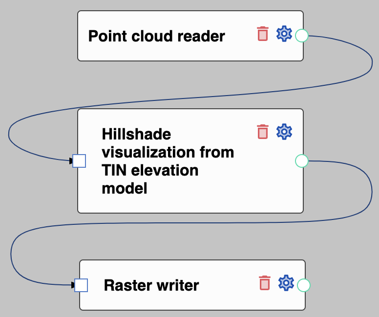
Flow to produce ground hillshade visualisation
All those steps are conveniently packed in a single processor node that can be used as part of the Flai processing flow (see our blog post for a longer description of how to create flows). From the available processors, select the node Hillshade visualization from the TIN elevation model and connect it to the point cloud reader and raster writer nodes. Its predefined settings should be adequate and left unchanged unless you need a finer resolution or want to visualize a different classification that default label 2 which is common from point cloud, classified as ground.
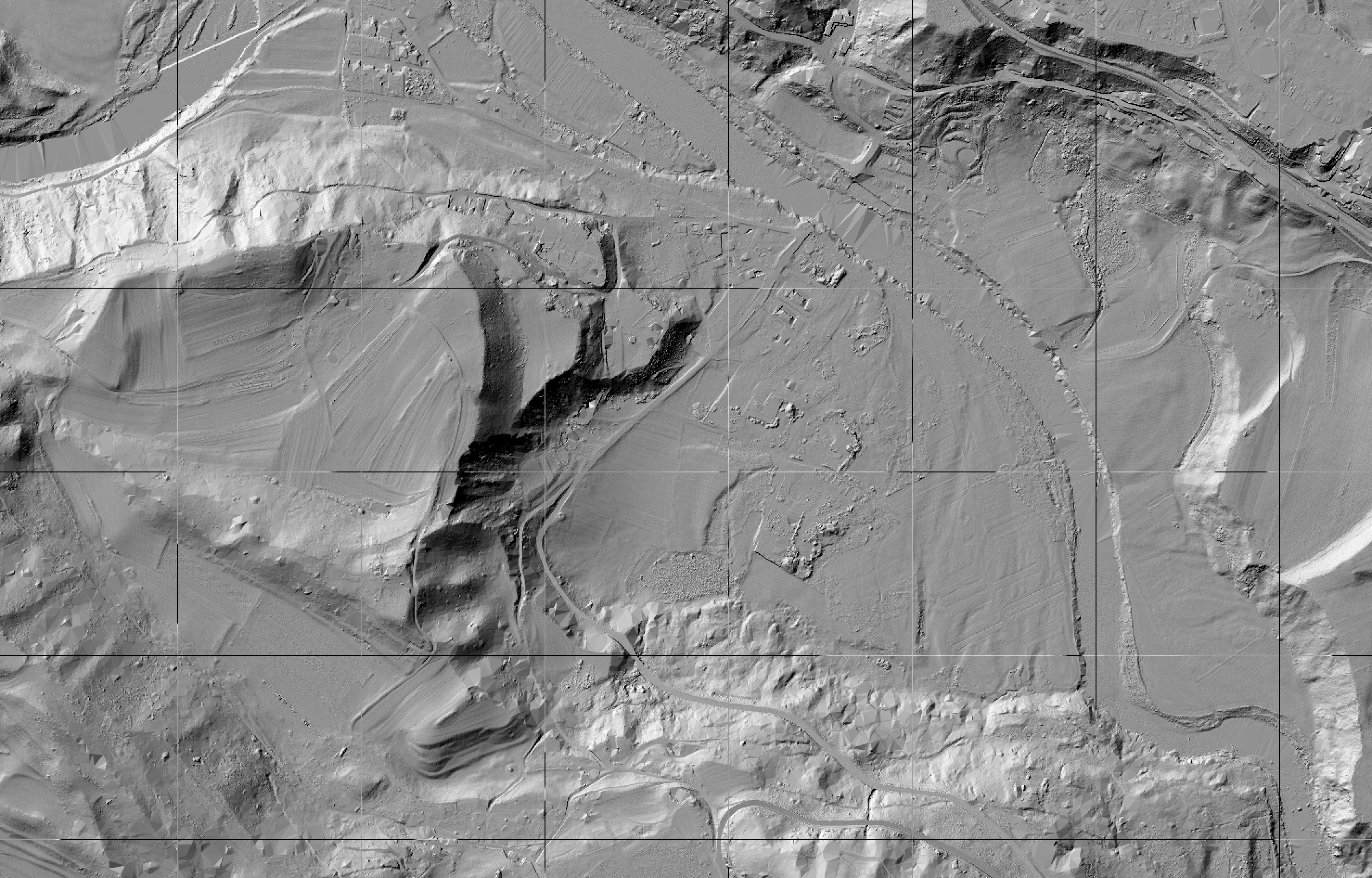
Example of created ground hillshade visualization. Grid lines represent borders between files in the dataset where shading operation is not well defined.
Rough object location and height mapping
If you ever need to produce a very rough map of objects that you are interested in and their height, you can use processor node Map class location by height for this task. The node allows you to specify a classification label, the size of produced pixels and possibly multiple height bins into which results are grouped. The height of an object is computed from above the ground. If the digital ground elevation model dataset is not supplied as one of the node inputs, it will be computed on-the-fly using points with a predefined classification label ground (2).
The result of this node is a raster with pixel values of 0 where no points coincide with the selected label. For the pixels whose perimeter encircles at least one point, they are assigned a value of the top bin range into which the highest point falls into. As such maps can look a bit patchy, they are at the end polished by the smoothing operator which removes small solitary detection and fills small holes.
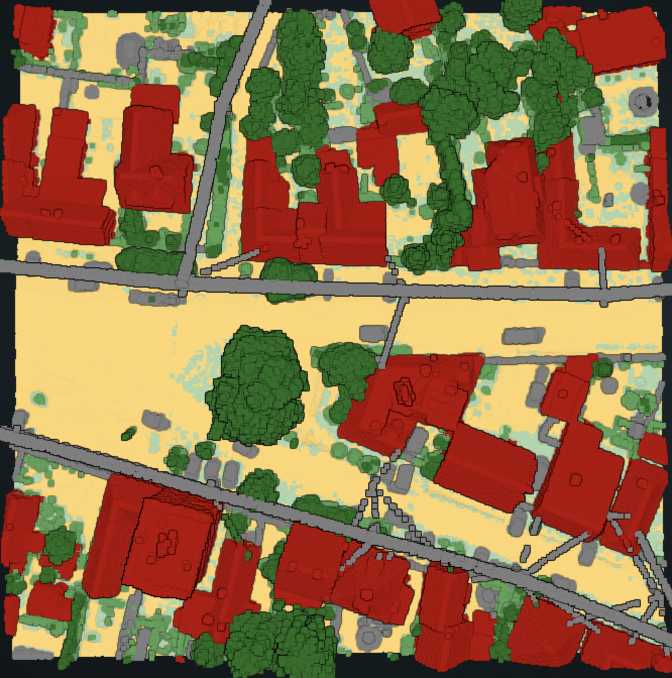
Input point cloud
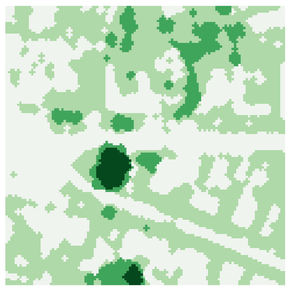
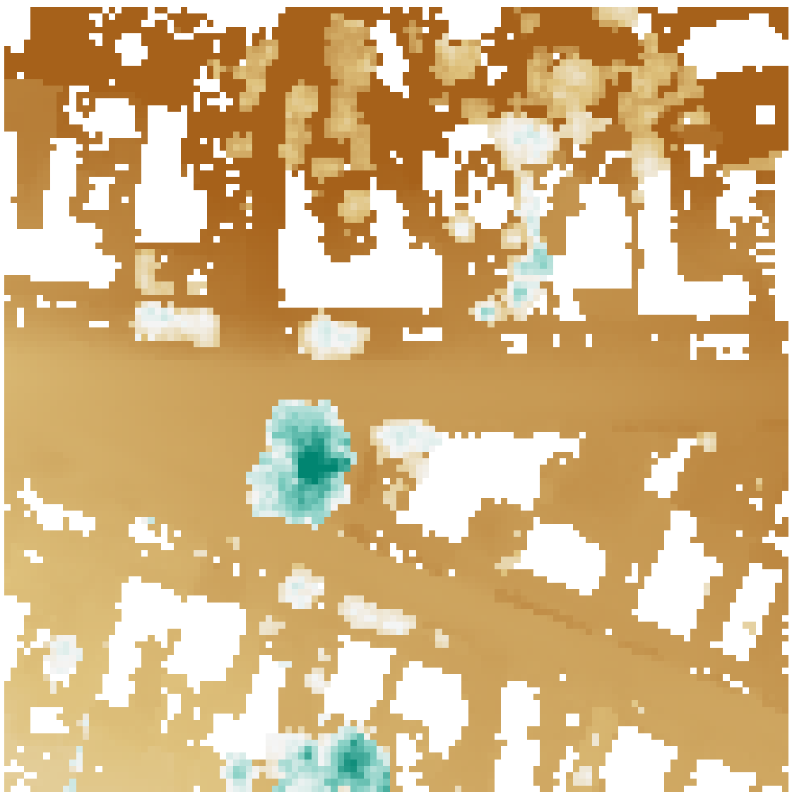
Created vegetation map
Example: The above images present the result of mapping vegetation location on our Demo dataset which is preloaded on sign-up. The processor was tasked with mapping vegetation (combined labels 3, 4 and 5 in the given dataset). We wanted to know the locations of potentially dangerous vegetation above 10 m. Therefore, we wanted to map vegetation location in three separate bins, 0-5 m, 5-10 m and 10-infinity m. To replicate the result, the node options for height above ground segmentation brackets would have to be written as [0:5], [5:10], [10:100]. Note that every bracket needs an upper and lower limit, and points that do not fall in any of them are discarded.
Advanced raster generation
Whenever you need more control over how rasters are generated or want to create custom products such as elevation or surface models, then you should use our processing node Rasterize point cloud. The node has numerous optional input parameters that are listed below in the same order as they appear in the web interface:
Pixel resolution controls the size of pixels and is given in the same units as the input point cloud.
The next option allows you to rasterize the value of any lidar attribute that is present in a dataset. The most common options are probably height z and intensity.
The output size allows you to control the spatial size of produced raster. When a single value is given, the output will produce square tiles of a given size. Instead, when option same is retained, the output rasters will be of the same size as point cloud files. Note that when you want to combine produced raster layers and their source point cloud in another processing node, option same must be used here.
The bounding extent of the output layer comes into play only when an integer value is given for image output size. It controls the area in which rasters are created. When left empty, all available rasters are produced and starting point of the grid is set to 0, 0 coordinates.
You can also control how many points per raster pixel are used to compute its value. The setting can be an exact value, selecting the desired number of closest neighbours or radial query. When a radius value is given, all points in the radius around a pixel centre are considered. If none of them is given, a query radius is computed from pixel resolution.
Attributes of selected points are reduced and aggregated into a single value by different approaches: IDW, min, max, mean, median, mode or percentile. There is also an option to only count the number of matching points per pixel or create a binary mask that marks where at least one point per pixel was present.
If you request percentile aggregation mode, there is also an option to set percentile value between 0 and 100%.
By default, all pixels without created value (no data pixels) are marked with the nan value, but this can be set to any value that you want.
Usually, we do not want to use all points in our dataset for rasterization. Their range can be specified by combining multiple lidar attribute filters. Filters of the same attribute are combined using OR operation and AND is used among filters of different attributes.
Colorized height model
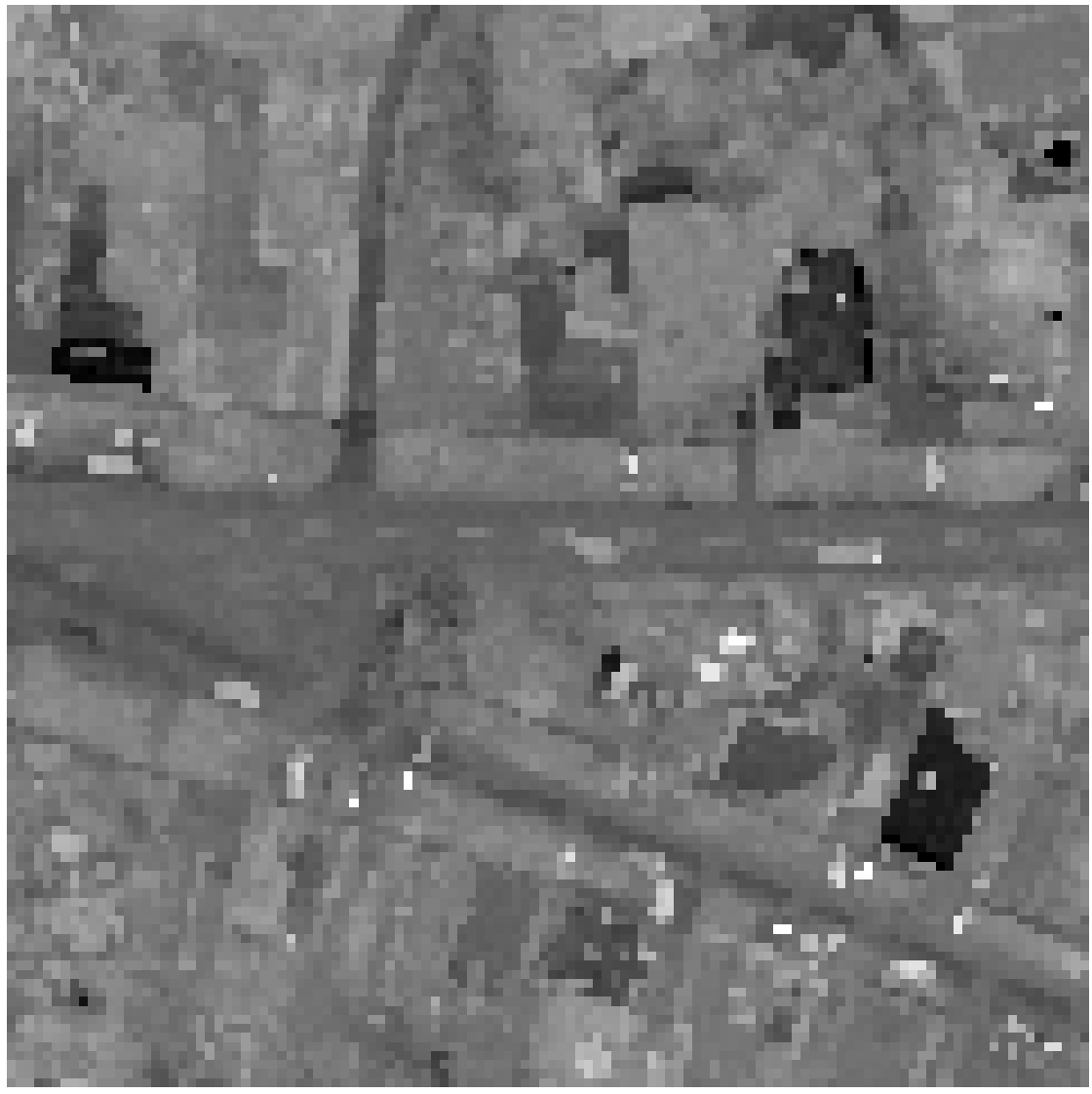
Grayscale maximal intensity
Left image: I want to rasterise the median height of pixels with classification labels of 2 and 5, whose intensity is lower than 27000. To produce this query, select z as the lidar attribute, choose the median reduction method and write the selection filter as Classification[2:2], Intensity[0:27000], Classification[5:5]. Right image: I want to create a max intensity value, regardless of the classification label. To produce this query select intensity as the lidar attribute, choose the max reduction method and clear any selection filters.
Missing pixel interpolation
Not all rasterization methods will produce a raster where every pixel is filled by some value. To fill the missing pixels, use a conveniently named processing node Interpolate no data pixels whose function is to fill missing information by nearby pixel interpolation. By default, this node will only fill pixels with nan and inf values. A range of interpolation complexity, from simple piecewise linear to complex bicubic, can be used. The input and output of the node are raster datasets.
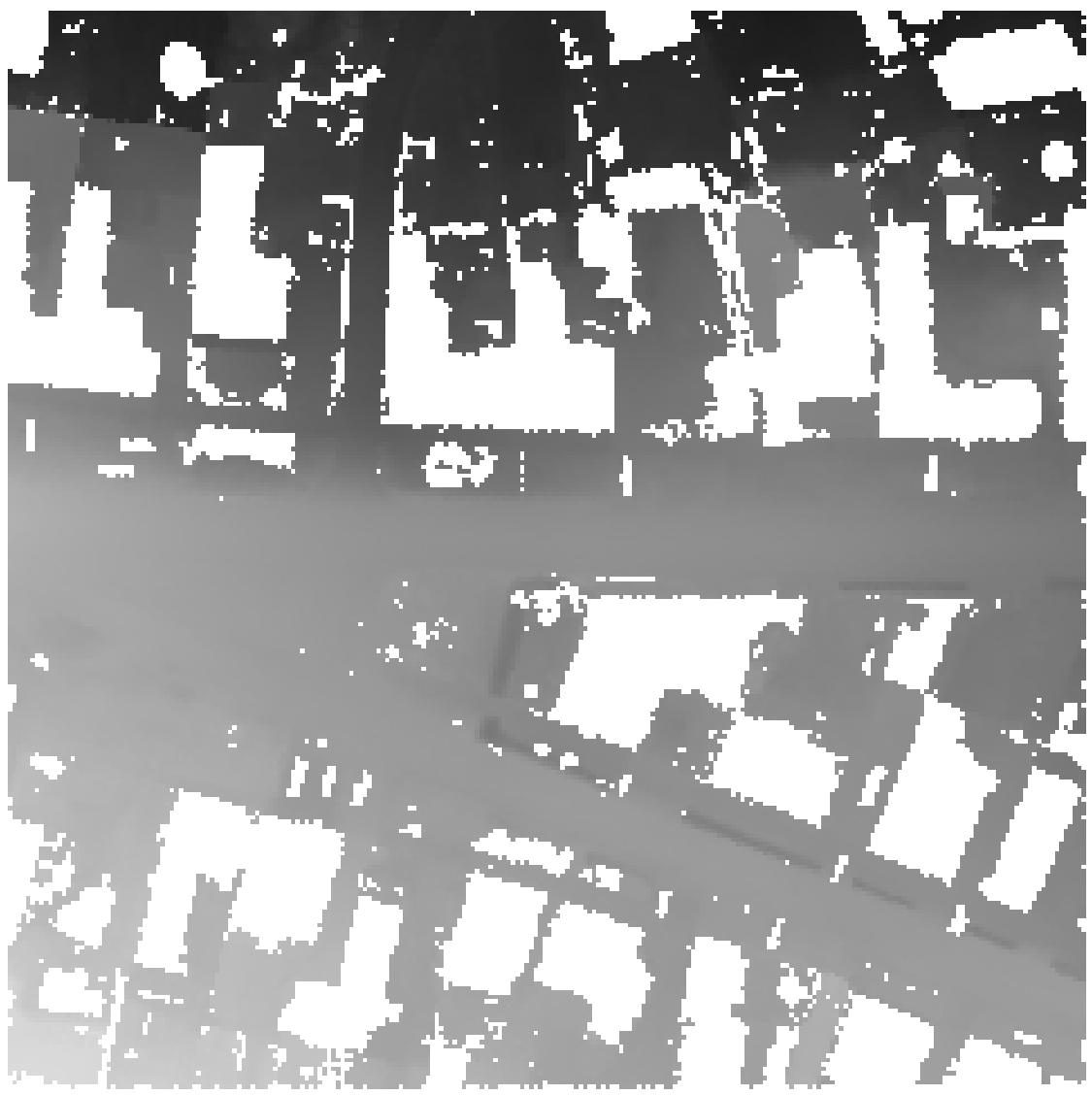
DEM before interpolation
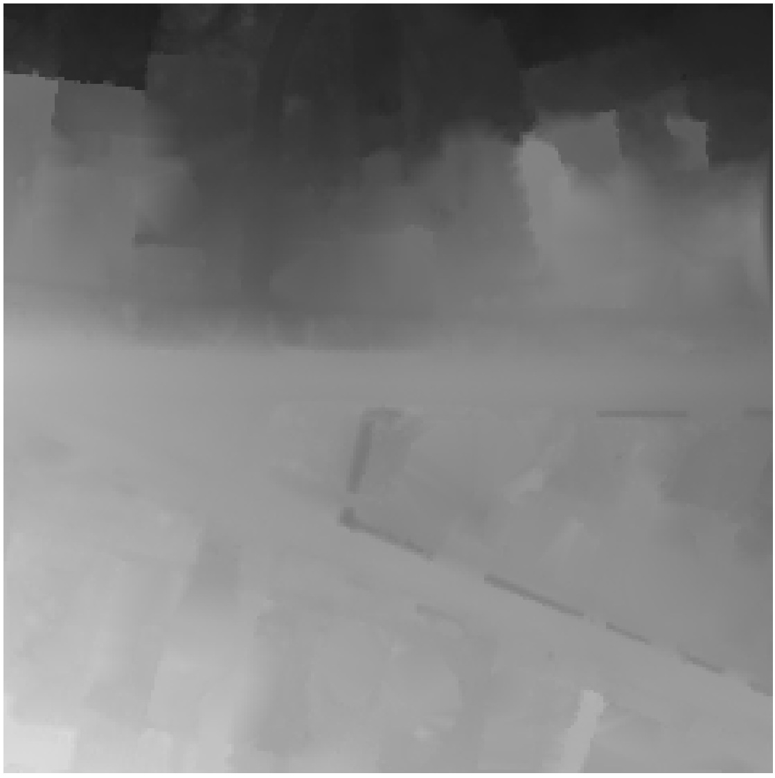
DEM after interpolation
Downloading the results
It is possible to download created rasters in the .tif file format by clicking the download icon for the selected Dataset in the Catalogue view. Once the download is prepared you will receive an email notification with the download link to the file.
Try our Flai web application
Tags:
Recent Posts
How to Keep Original (Ground) Labels Unchanged When Using Flai Classification
Pushing the Boundaries of Situational Awareness at REPMUS 2025: Our AI-Driven REA Journey